Electromagnetism – Life in Physics…

1) DoF of Graviton or more precisely, modes of $g_{\mu\nu}(x)$ (because nothing is quantized here!):

Let us start by writing $g_{\mu\nu}(x)=\eta_{\mu\nu}+\kappa h_{\mu\nu}(x)$ , where $\kappa^2=\frac{8\pi G}{c^4}$ . With this definition, Einstein’s field equation at linearized level becomes:

$G_{\mu\nu}^{lin}=-\kappa^2 T_{\mu\nu}^{(2)}$

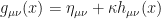
where the RHS refers to quadratic part of the Energy-Momentum tensor. For counting physical modes, we need to consider gravitational field without any sources so we will deal with just[1,2]:

$G_{\mu\nu}^{lin}=\frac{\kappa}{2}\left[\square h_{\mu\nu}-h_{\mu,\nu}-h_{\nu,\mu}+h_{,\mu\nu}-\eta_{\mu\nu}\left(\square h-h_{\alpha}^{,\alpha}\right)\right]=0$

where $h_{\mu}=\partial^{\nu}h_{\mu\nu}~\mathrm{and}~h=\eta^{\mu\nu}h_{\mu\nu}$ . This linearized field equation is invariant under the following gauge transformation:

$\delta h_{\mu\nu}=\partial_{\mu}\xi_{\nu}+\partial_{\nu}\xi_{\mu}$

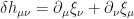
which is just the linearized version of the Einstein (general coordinate) transformation of the metric, $\delta g_{\mu\nu}=\xi^{\alpha}\partial_{\alpha}g_{\mu\nu}+g_{\alpha\nu}\partial_{\mu}\xi^{\alpha}+g_{\mu\alpha}\partial_{\nu}\xi^{\alpha}$ !

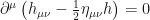
Now, as is usually done, we choose a gauge called de Donder gauge[3]: $\partial^{\mu}\left(h_{\mu\nu}-\frac{1}{2}\eta_{\mu\nu}h\right)=0$ . With this gauge choice and defining $\phi_{\mu\nu}=h_{\mu\nu}-\frac{1}{2}\eta_{\mu\nu}h$ , we get the following redefined equations:

Field Equation: $G_{\mu\nu}^{lin}=\frac{\kappa}{2}\square \phi_{\mu\nu}=0$

de Donder Gauge: $\partial^{\mu}\phi_{\mu\nu}=0$

Gauge Transformation: $\delta\phi_{\mu\nu}=\partial_{\mu}\xi_{\nu}+\partial_{\nu}\xi_{\mu}-\eta_{\mu\nu}\partial_{\alpha}\xi^{\alpha}$

Let us choose a plane wave solution for the field equation: $\phi_{\mu\nu}=\epsilon_{\mu\nu} e^{i k.x}$ . First thing to note is that $\phi_{\mu\nu}$ has 10 components/modes (in 4-D obviously!). The question is how many of them are physical modes. You probably already know the answer but we’ll get there slowly but concretely! Let us plug the solution in the first two equations above to get:

$\square\phi_{\mu\nu} = -k^2\phi_{\mu\nu}=0 \Rightarrow k^2=0$

$\partial^{\mu}\phi_{\mu\nu}=0 \Rightarrow k^{\mu}\epsilon_{\mu\nu}=0$

The last equation reduces the number of independent modes in $\phi_{\mu\nu}$ to 10-4=6. We have the following 6 ‘most general’ basis tensors for $\epsilon_{\mu\nu}$ assuming wave propagation is in 3(z)-direction, i.e. $k_{\mu}=(-1,0,0,1)$ :

$1.~\epsilon_{1\mu}\epsilon_{1\nu}+\epsilon_{2\mu}\epsilon_{2\nu}$ ,

$2.~\epsilon_{1\mu}\epsilon_{1\nu}-\epsilon_{2\mu}\epsilon_{2\nu}$ ,

$3.~\epsilon_{1\mu}\epsilon_{2\nu}+\epsilon_{1\nu}\epsilon_{2\mu}$ ,

$4.~\epsilon_{1\mu}k_{\nu}+\epsilon_{1\nu}k_{\mu}$ ,

$5.~\epsilon_{2\mu}k_{\nu}+\epsilon_{2\nu}k_{\mu}$ and

$6.~k_{\mu}k_{\nu}$ .

where $\epsilon_{1\nu}=\delta^{\mu}_{1}\epsilon_{\mu\nu}$ and so on. Let us now look at the gauge transformation of $\epsilon_{\mu\nu}$ after choosing a specific form of the gauge parameter, $\xi_{\mu}=C a_{\mu}e^{i k.x}$ (where C is a constant which could be absorbed in $a_{\mu}$ !):

$\epsilon_{\mu\nu}^{\prime} = \epsilon_{\mu\nu}+i C\left(a_{\mu}k_{\nu}+a_{\nu}k_{\mu}-\eta_{\mu\nu}a_{\alpha}k^{\alpha}\right)$ .

As we did for $\epsilon_{\mu\nu}$ , the most general basis vectors for $a_{\mu}$ are chosen to be $\epsilon_{1\mu}, \epsilon_{2\mu}, k_{\mu}~\&~\bar{k}_{\mu}=(1,0,0,1)$ . We immediately see that the choice of first three basis vectors and a ‘correct’ C makes the modes 4, 5 & 6 pure gauge i.e. $\epsilon^{\prime}=0$ . Last basis vector is a bit tricky, so let us look at this tricky identity:

$\eta_{\mu\nu}=\epsilon_{1\mu}\epsilon_{1\nu}+\epsilon_{2\mu}\epsilon_{2\nu}+\frac{\bar{k}_{\mu}k_{\nu}+\bar{k}_{\nu}k_{\mu}}{\bar{k}_{\alpha}k^{\alpha}}$ ,

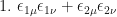
And you immediately ‘see’ that (with ‘correct’ C) the mode which is gauged away is 1! So we are left with 6-4=2 physical modes:

$\epsilon^{+}_{\mu\nu}=\epsilon_{1\mu}\epsilon_{1\nu}-\epsilon_{2\mu}\epsilon_{2\nu}~\mathrm{and}~\epsilon^{\times}_{\mu\nu}=\epsilon_{1\mu}\epsilon_{2\nu}+\epsilon_{1\nu}\epsilon_{2\mu}$ .

These are the two ‘famous’ plus- & cross- modes/polarizations of the gravitational waves.

***

2) DoF of Photon or more precisely, modes of $A_{\mu}(x)$ :

The Maxwell’s equation of motion is as follows:

$\square A_{\mu}-\partial_{\mu}\partial^{\nu}A_{\nu}=0$ .

This equation is invariant under the following gauge transformation:

$\delta A_{\mu}=\partial_{\mu}\lambda$ .

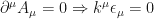
Now, we choose a gauge called Lorentz gauge:

$\partial^{\mu}A_{\mu}=0$ .

With this gauge choice, we get the following simplified equation of motion:

$\square A_{\mu}=0$ .

Let us choose a plane wave solution for this equation: $A_{\mu}=\epsilon_{\mu} e^{i k.x}$ . Firstly, $A_{\mu}$ has 4 components/modes (in 4-D!). Plugging this solution in the two equations above, we get:

$\square A_{\mu} = -k^2 A_{\mu}=0 \Rightarrow k^2=0$

$\partial^{\mu}A_{\mu}=0 \Rightarrow k^{\mu}\epsilon_{\mu}=0$

The last equation reduces the number of independent modes in $A_{\mu}$ to 4-1=3. We have the following 3 ‘most general’ basis vectors for $\epsilon_{\mu}$ (assuming wave propagates in 3(z)-direction):

$1.~\delta^{1}_{\mu}$ ,

$2.~\delta^{2}_{\mu}$ and

$3.~k_{\mu}$ .

Let us now look at the gauge transformation of $\epsilon_{\mu}$ after choosing a specific form of the gauge parameter: $\lambda=C e^{i k.x}$ (where C is a constant!) which gives:

$\epsilon_{\mu}^{\prime} = \epsilon_{\mu}+i C k_{\mu}$ .

We immediately see that a ‘correct’ C makes the mode 3 pure gauge. So we are left with 3-1=2 physical modes:

$\epsilon^{x}_{\mu}=\delta^{1}_{\mu}~\mathrm{and}~\epsilon^{y}_{\mu}=\delta^{2}_{\mu}$

These are the two ‘famous’ linear modes/polarizations of the electromagnetic waves.

———

[1] If you are wondering which action gives that field equation, it is just the quadratic part of the Hilbert-Einstein action (which is proportional to the Fierz-Pauli action for spin-2 particle): ${\cal L}_{H-E}^{(2)}=-\frac{1}{2}\left[\frac{1}{4}h_{\mu\nu,\rho}^2-\frac{1}{2}h_{\mu}^2+\frac{1}{2}h^{\mu}h_{,\mu}-\frac{1}{4}h_{,\mu}^2\right]$ .

[2] There are many subtleties involving $T_{\mu\nu}$ in GR and you are welcome to read S. Weinberg’s ‘Gravitation & Cosmology’. Also this .pdf file covers Second & First Order formalism in an irritating manner but is quite good nonetheless!

[3] You can do a similar analysis as was done in the previous post for the case of Maxwell’s EM theory for choosing this particular gauge condition.

Life in Physics…

Category: Electromagnetism

Physical DoF of Graviton & Photon(revised)