To Explain the World

Today is Ed Witten’s birthday, apparently. I recently completed S. Weinberg’s book “To Explain the World”, so I will instead collect some excerpts from that book here. Let’s start with one from near the beginning of the book.

There remains a poetic element in modern physics. We do not write in poetry; much of the writing of physicists barely reaches the level of prose. But we seek beauty in our theories, and use aesthetic judgments as a guide in our research.

I like the phrase “barely reaches the level of prose”. It really made me laugh out loud, while reminding me of a quote by Francis Crick:

There is no form of prose more difficult to understand and more tedious to read than the average scientific paper.

Moving on, Weinberg also cites the preface to the “Treatise on Light” by C. Huygens:

There will be seen [in this book] demonstrations of those kinds which do not produce as great a certitude as those of Geometry, and which differ much therefrom, since whereas the Geometers prove their Propositions by fixed and incontestable Principles, here the Principles are verified by the conclusions to be drawn from them; the nature of these things not allowing of this being done otherwise.

I like this “way of doing science” as it is how I think about theoretical physics research, especially high energy physics. Of course, the sentiment above is as valid for any theorist or experimentalist or phenomenologist or someone in-between. Because in my view, the phrase “⋯Principles are verified by the conclusions⋯” is so broad that the “conclusions” include everything from experimental results (Gedanken or physical or any other kind one could think of) to results in terms of equations (Abstract or useful or any other kind one could think of). This broad view further enforced by the next phrase “⋯nature of these things not allowing of this being done otherwise”, puts into perspective that the “dated” view of scientific method (Hypothesis → Experiment → Confirmation? → Theory or Re-Hypothesize!) is indeed “dated”. The scientific method should instead be thought of as “Principles → ??? → Consequences”. [A better discussion along similar lines can be found here.] The “???” could be anything from a one-page mathematical proof to a simple thought-experiment to a backyard contraption to a billion-dollar lab experiment to a decades-long development of a theoretical framework. The former view of a scientific method is good enough to be discussed in a nursery class where kids don’t even realize that something could be subtracted from 0 whereas the latter is what actually happens in the real world of scientific research. Though, even the real researchers could be in denial of this fact most of the time, because the early nursery education is quite hard to override, even by the time one becomes a faculty member. A personal example of this: after I finished my talk on “3d supersymmetric localization” at SNBose and asked one of the senior professors what he thought about the talk, he replied, “I am a real physicist”! I laughed out loud, and thought, “Oh, he’s that kind of a physicist!”. By “that kind” I, of course, mean someone who hasn’t been able to move past the above-mentioned nursery education.

Someone at this point will surely interject and say something like, “what about the real world?” or “what about this thing’s usefulness?” or “what about the real world applications?” or “when will I actually need this in my real life?”. For all those interjectors, I point my index finger towards the future posts which I will write on this blog slowly and steadily, but surely, as I continue burning various bridges. Because why not? In short, here are my two cents: Have you seen the real world recently? Why the hell would I ever think about it, except in my nightmares? Supersymmetry and Superspace is a much better and nicer place to live in and it turns out to be quite useful to avoid the real world, and that’s all I need in my real life!

That went off in a different direction than intended so let’s get back on track with another excerpt from the book.

The search for knowledge of practical value can serve as a corrective to uncontrolled speculation, but explaining the world has value in itself, whether or not it leads directly to anything useful.

This again echoes what I said above or rather, what I said above echoes these thoughts of Weinberg. Of course, it’s the latter.

We get intense pleasure when something has been successfully explained, as when Newton explained Kepler’s laws of planetary motion along with much else. The scientific theories and methods that survive are those that provide such pleasure, whether or not they fit any preexisting model of how science ought to be done.

Weinberg so eloquently expresses the need to throw away the “outdated” view of the scientific method, which according to him, had outlived its usefulness already at the time of Newton. And finally,

The rejection of Newton’s theories by the followers of Descartes and Leibniz suggests a moral for the practice of science: it is never safe simply to reject a theory that has as many impressive successes in accounting for observation as Newton’s had. Successful theories may work for reasons not understood by their creators, and they always turn out to be approximations to more successful theories, but they are never simply mistakes.

Well-said but it seems this moral is not taken seriously even by many self-appointed real physicists in this day and age!

That’s quite a long post which I definitely did not intend for it to be. So let’s leave it there, as I move on to another book of Weinberg:

Third Thoughts

Communicating Science Challenge

4gravitons has proposed a challenge: To explain scientific papers appearing on arXiv on a given day in a given (sub)field to a general audience. The challenge is directed towards fellow science communicators so that definitely excludes me. But one of my old year thoughts (turned to a new year resolution) for this blog was to discuss papers on arXiv that interested me, on a monthly basis (apart from some physic(ist)s-related rants like this) in an effort to keep this blog (sort of) active. So, despite not being a science communicator, I feel like the above-mentioned challenge is one way to get into discussing papers this month. So here we go…

Warning as given by 4gravitons: I’m looking at papers in the “High Energy Physics – Theory” area, announced 10 Jan, 2022. I haven’t read these papers, just their abstracts, so apologies if I got your paper wrong!

Extra Disclaimer: I am not an expert in any of the (sub)topics covered by the 11 papers appearing below. I am familiar with enough ‘hep-th jargon’ to have a vague idea about what each paper might be about and that’s what is reflected in my explanations. So don’t take what follows too seriously, or to put it another way, take it seriously at your own risk.

[1] arXiv:2201.02200: A p-Adic Matter in a Closed Universe

The author looks at dynamics of an exotic kind of matter and its implications to cosmology. They find by employing Einstein’s theory of gravity that a Universe filled with this kind of matter would be closed (like the surface of a sphere) and would expand exponentially. They also discuss the possibility of this kind of matter as a dark matter candidate. [Our Universe with ordinary + dark matter (+dark energy) is more or less flat and expanding but not exponentially.]

[2] arXiv:2201.02201: Anisotropic Special Relativity

Einstein’s theory of Special Relativity treats all directions of space and time on equal footing. As the title of this paper suggests, the author here considers breaking the isotropy of space and choosing one preferred direction in space. Using such a setup, they go on to discuss the consequences for quantum field theory, which is the framework used to describe our current understanding of fundamental particles and forces known as the Standard Model. [Not sure how far they reach in ‘reworking’ QFT using ASR as I’ve not read the paper.]

[3] arXiv:2201.02206: Precision Bootstrap for the \mathcal{N}=1 Super-Ising Model

This is a note detailing a computational technique used to determine some physical properties of a 3d lattice of ‘spins’ (variables that can take two values like {+1, -1}) in a better way than previously used techniques. Such 3d systems are useful in studying phase transitions (like ice → water → steam), modelling phenomena like ferromagnetism, spin glasses, and even neurons! So having the ability to compute stuff easily and efficiently is always welcome. [I don’t think I can make it any more interesting.]

[4] arXiv:2201.02407: More on Topological Hydrodynamic Modes

The authors discuss fluid/gravity correspondence, a version of holography where fluid dynamics (or hydrodynamics) is described by a gravity theory living in one dimension higher. Specifically, they find a holographic description of a hydrodynamic phenomenon they had discovered earlier. What they had discovered were special kind of very-low-energy (virtually zero) fluid excitations (or modes) by ‘weakly’ breaking energy-momentum conservation in the hydrodynamic system. In this paper, by choosing a special rotating frame of reference (think of a merry-go-round; using Einstein’s equivalence principle, this rotating system can be thought of as a non-rotating system with a gravitational force), they could find existence of the same very-low-energy modes in the holographic setup too. They also extend their holographic construction to include ‘electric’ charges and find similar very-low-energy modes. [Usually, any paper whose title starts with “More on” or “Note on” is more or less an addendum to a previous paper without much of an independent story. I have also been known to succumb to this practice more than once in the past and will do so again later this year.]

[5] arXiv:2201.02412: U(1) Fields from Qubits: an Approach via D-theory Algebra

A framework for building algorithms for quantum computing is being explored in this paper. The authors pick a simple quantum mechanical toy model and discuss ideas to extend it to more complex models in various dimensions ranging from 1d to 4d (our world). One of the motivations for considering this seems to be the possible generalization to QCD (quantum chromodynamics; the theoretical framework describing strong nuclear force where exact analytical calculations are quite hard to perform and usually discretized spacetime lattices are used to perform calculations that are expected to give sensible answers in a continuum limit) such that lattice computations for QCD become more ‘robust’. [Don’t know why but this paper reminded me of one of my parody papers that I wrote ages ago, where one simple equation surprisingly described all of physics!]

[6] arXiv:2201.02493: Solving formally the Auxiliary System of O(N) Non Linear Sigma Model

I don’t think I’ll attempt to explain this. Can someone else give it a try? [What? I’m still only at the half-way mark… Man, this is harder than I expected even after taking into account that explaining things is hard!]

[7] arXiv:2201.02500: Entanglement Entropy in Horndeski Gravity

Entanglement Entropy is a measure of quantum entanglement between two subsystems of a quantum system. Holographic EE is a quantity computed for a certain gravitational system by considering a subregion in a spacetime with boundary, which encodes the EE of a non-gravitational matter system living on that boundary (with the two subsystems required for EE being the chosen subregion on the boundary and the rest of the boundary). The author chooses a general theory of 4d gravity (Horndeski) and computes HEE for an infinite strip subregion of the boundary. Certain information theoretical and thermodynamical aspects of this setup are then discussed. [Isn’t it always a good idea to refrain from citing papers in the abstract? I have been guilty of doing that myself but that one was unavoidable!]

[8] arXiv:2201.02524: On some new types of membrane solutions

The author provides new solutions (of certain extensions of Einstein’s equations of gravity) in M-theory (mother of all string theories) with two time dimensions and discusses their properties, like no black hole formation. [Usually, one deals with only one time dimension.]

[9] arXiv:2201.02572: Topological invariant of 4-manifolds based on a 3-group

This paper claims to be a generalization of another paper from 2007, which has been flagged in the “arXiv admin note”. Anyway, the authors consider an exotic extension of Maxwell’s theory of electromagnetism to study properties of 4d spacetimes. They construct a quantity ‘Z’ which is a topological invariant, by which it is meant that this Z does not depend on the specifics of the 4d spacetimes (for example, how distances are measured on them) but just on the overall shape (topology) of the spacetime. In a certain sense, it means that Z can be used to classify different types of 4d spacetimes (for example, 2d surfaces can be classified by counting the number of holes). [Also note that they give a nice way to avoid using citations in the abstract!]

[10] arXiv:2201.02575: The spatial Functional Renormalization Group and Hadamard states on cosmological spacetimes

The authors study the ‘flow’ of a special state living on cosmologically relevant spatial and temporal scales. They give a concrete mathematical realization of such a state and study how the state flows from high energy (ultraviolet; let’s say near Big Bang) to low energy (infrared; let’s say our humdrum life now). They find that choosing certain states of low energy in pre-inflationary period (inflation is the epoch of exponential expansion in our cosmological past, very close to the Big Bang) and allowing them to flow using their ‘flow equations’ leads to concretely computable property of the state in the kind of spacetime that we are familiar with now!  [So many familiar words, yet their exact order renders them challenging to comprehend! Hopefully, I have gotten the gist of the abstract right.]

[11] arXiv:2201.02595: Celestial holography meets twisted holography: 4d amplitudes from chiral correlators

This paper introduces a new program for computing scattering amplitudes (actually, certain parts of it; the whole thing is expected to give the probability for a given scattering event to take place) in 4d field theories (involving photons, W/Z bosons, gravitons, etc.) from certain 6d theories. They recognize these parts of the scattering amplitudes as something originating in different kinds of 4d theories and/or 2d theories. This connection allows them to reproduce well-known results efficiently as well as compute some new results for certain scattering amplitudes. In addition, they also make contact with other programs like “celestial holography” and “twisted holography” that have become quite popular recently. [For the last statement, I refer to my previous post reviewing ISM 2021 and links therein.]

ISM 2021 Review

The past week saw 6 days of the latest edition of “Indian Strings Meeting” hosted by IIT Roorkee. Well, more like hosted by Aalok Misra with some background support from his ‘tech team’ taking care of Zoom calls and YouTube live streams and Webpage updates. I could not attend the Zcalls because of connection problems (at my end I guess) as audio and/or shared screen would randomly drop so I mostly watched the YT live streams. The latter was quite a barren region with <20 viewers at any given time compared to the former which was bustling with <50 participants (i.e., whenever I could join and see and hear something relevant). I wonder what happened to the ~400 registered participants on the website!

Anyway, enough with the personnel logistics, let’s get on with the real logistics that is most relevant in a conference review. That of how many talks were there and of what kind. I will categorize the talks based on four topics extracted from the six review talks, two more topics for 3d field theories and non-3d field theories and one last ‘miscellaneous’ topic (as expected) to catch all those that do not fit into the aforementioned six topics. I do feel like I should mention a disclaimer here, before we have a look at the table, that this categorization of talks is my personal subjective opinion and not to be taken as that of the speakers or Aalok or ISM’s NOC or anyone else for that matter. If anyone does not agree with this categorization, they are welcome to comment below or write their own post and share it as a comment below. (No guarantee that it will change my opinion but if it does, I will be happy to edit things around here accordingly.) Here goes the full table with raw data mined from here:

Topic Review Talks (60m) Research Talks (30m) Short Presentations (15m) Total Time (h)
(A)dS/CFT + Holography RG1 + EP6 + DG6 = 3 TT1 + KN1 + SA2 + SD2 + RL3 + KS3 = 6 SM6 + AS6 = 2
BMS Symmetry + Flat Space Holography LD2 CK1 + AB2 + MM2 + AB2 + RB4 + AYS5 + PP5 = 7 PP5 + DG6 = 2 5
Black Holes + Information Theory DH3 AM1 + AV2 + OP3 + DS3 + NK4 + AA4 + PR6 + JC6 + JKB6 + RS6 + SP6 = 11 AK1 + AKP2 + SM2 + SK3 + AG4 + HP4 + GB5 + AB5 = 8
Amplitudes + (OTO) Correlators JP6 AK1 + AZ1 + AS3 + AR5 + AM5 + SK6 = 6 SD1 + APS1 + SK2 + TS3 + PH5 + AM6 = 6
3d (S)CFTs AM1 + SG2 + KC2 + SM3 + SJ5 = 5 RRJ1 + NP4 = 2 3
Other Field Theories RG2 + YT3 + CG3 + ZK3 + SD4 + VBS4 + NS4 = 7 DM4
Miscellaneous AM1 + BS3 + SG3 + KR5 + LA5 + NS5 + AM6 = 7 MS3 + MM3 = 2 4
Total: 6 49 23 36¼

Let’s acknowledge that the notation used in the table is self-explanatory: the letters are the initials of the speakers (no effort is put to break the degeneracy of AM’s, et al) and the number denotes the day on which they spoke. I have doubly cross-checked the data on the official webpage and my categorization above for consistency. Normally, I don’t put anything up on my blogs, unless it is quadruply checked but since even the official data is not rigorously vetted, I don’t think I need to exert myself that much in this post. For example, a speaker (Parijat Dey from Uppsala University, Sweden) appears in the detailed list of talks but not in the schedule table, which I guess happened because two speakers cancelled their talks on the fifth day which were then moved to the sixth day! Also, at least one 15m talk appears in the list of 30m talks (or vice-versa) and of course, the big elephant in the room is that Enrico Pajer’s hour-long review talk appears in a 30m timeslot and it was treated as something in-between! So given that the raw data is not too trustworthy, I think the doubly checked table appearing above is more than enough for my purposes here.

I also have some pet peeves about the formatting/styling employed for the “Schedule” webpage linked above. I mean, who in the ‘tech team’ had the ‘brilliant’ idea of sorting the detailed list of talks wrt length of the talks and then further sorting alphabetically (which is also not quite correct) wrt last names of the speakers? This leads to the following bad user experience: when someone clicks a speaker’s name in a particular timeslot of the schedule table, they are catapulted at warp-speeds through the long webpage to the speaker details but now they’re lost (& disoriented) because they don’t see any other speaker details around the timeslot they were just looking at a moment ago! This problem could have been avoided if the speakers were sorted chronologically and not alphabetically (basically, focus on talks and not speakers). Also, that awfully long webpage could have been shortened by light-years if a tabbed interface were used for the six days, with each day’s tab showing the chronological details of the talks. I also find the insistence on “speakers of” review/research talks in the headings for the corresponding sections but not for the short presentations pretty hilarious (see the screenshot below). As if the people giving those short presentations are not worthy of being even identified with a common noun. Talk about inequalities prevalent in academia! This problem also would not have risen if the talks were chronologically listed. A lot fixed with a simple change in one’s viewpoint.

ISM 2021 Speakers?

Anyway, enough of my rant about webpage development (I mean I could have done a better job myself of formatting/organizing that page… Come on, man! Move on! Your rant just spilled on to the next para… and I will have to start a new clean para again!).

That table above presents quite a boring view so let’s look at a colourful chart based on it instead:

Stacked Bar Chart 1

We see that the topic of black holes and related stuff like entanglement entropy, information paradox was extremely popular taking up more than eight hours, i.e., more than a day in a six-days-long conference. The three other main topics in this conference were “(A)dS/CFT & holography”, “S-matrices, scattering amplitudes & correlators (incl. OTOCs)”, and “BMS symmetry & flat space holography”, which took up roughly a day each. The talks on field theories in various dimensions took up another day with most people focussing on 3d (super)conformal field theories but some quite interesting talks on 2d and 4d theories too. Disappointingly, my personal favourite “5d SCFTs” barely got mentioned. Finally, the miscellany of talks included a talk on string phenomenology, a couple on constructing actions for Weyl supergravity multiplets, and a few on mathematical aspects like new Lie algebras, machine learning, etc. Before we move on, let us also see the above data split day-wise. Can you spot the only topic which was talked about every single day? The answer won’t surprise you!

Stacked Bar Chart 2

Now, I guess I should lay down my own personal views on ISM 2021. First (confession), I didn’t watch all the talks but most of them to be able to have some motivation to write this post. Second, the constant shifts of the schedule by at least 15m (and going up to 45m as the day progressed) really twisted my holography (reference to DG6’s talk if you don’t get my drift). Third, I was looking forward to some talks because of their titles, some because of their speakers. Both of these types didn’t disappoint. Others were hits and misses. Fourth, the constant bug in almost all of the talks was that typical questioner/commenter who hadn’t properly formulated (or even envisioned) the question before opening his (let’s be real, it’s definitely ‘his’ not ‘her’!) mouth, leading to mostly vague questions or tautological statements disguised as comments. That led in turn to more haw-ing, hmm-ing, “I mean(t)”’s, “you know, like”’s, “the the, so that thing”’s, “the usual thing, you know”’s, “so so, that’s what… the the, what I meant was”’s, etc. You get the idea why it bugged me, right? I wish Indian institutes had “graduate seminar courses” like I had at Stony Brook where professors actually gave you proper feedback on your talks. In addition, listening to fellow students in that ‘classroom’ setting made you aware of what to do and what not to do during talks, both yours and others. Some of the speakers & listeners of this conference could have definitely used some exposure to such a course. Fifth, I didn’t listen to most of the discussion sessions, except one where the bugging became quite unbearable and I just had to leave. I had better things to do like watching “Have I Got a Bit More News for You?” or having dinner or anything else.

Finally, we have to discuss what does all this mean. As in, what is the string theory research landscape in India like? Where is this research program headed in India? What are the differences compared to similar programs in other countries? And so on… I couldn’t care less about answering such boring questions. Indirect answers (or sketches thereof) to some of these questions are already available in the previous but one para. Even then, one ‘answer’ that just screams out of the data and charts above is: The ST research landscape is mostly covered by two (composite) peaks, those of black holes and (any kind of) holography. The two peaks from which I am as far away as possible given the plain areas of my research of the past decade. Let’s end this geological metaphor and get back on track of the un-punny sentences. My research falls majorly in the two minor categories of 3d (S)CFTs and other field theories (mostly dealing with 5d theories, as mentioned above) with some minor overlap with the major category of AdS/CFT & holography. As we all know, 2021 was not a good year for many reasons for many people, and I can now add this one revelation to my personal list of such reasons. This might urge one to ask so would I be moving towards the peaks from the plains? Oh, Hell No! I am quite happy with the plains I prowl on.

Wait, there’s one last thing to talk about: Discussion session on gender imbalance in STEM. I guess one of the reasons we have this problem is we talk about it at the end. Ok, enough with the jokes. This was a serious discussion… I learnt a lot with some precise language and data fleshing out the vague ideas I have had about the problem. The panelists in this discussion session represented ‘all walks of academic life’ who shared their experiences, talked about steps taken, being taken, steps in the pipeline, etc. Even general ideas encompassing treatment of minorities and amendment of systemic procedures to be more inclusive got an airing out. I encourage everyone to listen to this session, even re-listen, so that things (start to) change for the better.

Happy New Year! 🎉

Superspace

It has been a while since I posted anything on this WordPress blog. Since I’ve just bought a domain name from WordPress, I thought I should post something, even if just to mention this update in the blog’s address. But that’s just some filler content that I post on my other blog. So here I should at least talk about some Physics.

Superspace – the greatest invention since the wheel – is where I spent most of my graduate days. After graduating, I have spent less time there but I have regularly visited it over the years. Last year, I visited it to settle a 7 (or so) years old score with my collaborators by writing a paper on quantization of supersymmetric Yang-Mills theory in 4d \mathcal{N}=3 harmonic superspace that is actually useful in computing loop graphs.

Now, a popular physics blog would go to great lengths to try to explain to a layperson the various technical words that appear in the above paragraph, like quantization, SYM theory, \mathcal{N}=3, harmonic superspace, and loop graphs. [Of course, 4d just refers to our (3+1)-dimensional spacetime: 3 space and 1 time directions.] As it turns out, 4Gravitons is just that sort of a blog and most of these terms have been explained there: Quantization, Supersymmetric, Yang-Mills theory, \mathcal{N}=3 (well, \mathcal{N}=3 is quite similar to \mathcal{N}=4), Loop graphs.

The most astute reader amongst you must have already realized that harmonic superspace is not explained there. Or maybe, it has been but I have deliberately not linked to that page. The reason for doing that is quite simple: I am supposed to be the (second-)last ‘expert’ on harmonic and projective superspaces in the whole world. By “(next-to-)last ‘expert’ in the whole world”, I don’t mean the pejorative phrase “world-famous in India”, I literally mean the former phrase and it does not have any connotation about fame at all in it. So, being one of the ‘experts’ in superspace, I can’t link everything to 4Gravitons (who is an expert in another subfield of theoretical high energy physics) as I believe that one should undertake the undertaking about explaining something that one is an expert on to the lay-world.

Here goes my feeble attempt then. [Disclaimer: Anyone expecting clarity and thoughtfulness in crafting the explanations, as found at 4Gravitons, will be disappointed.] First of all, we must agree with the basic fact that harmonic superspace is a kind of a superspace. Then, we need to define a superspace and later we will tag on the adjective ‘harmonic’ in a hand-waving way, which should be sufficient for the level of this post.

A superspace is an extension of the usual spacetime x^{\mu}=(t,x,y,z) with extra coordinates which have no basis in reality. (There, I said it; no beating around the bush.) These coordinates are such that (let’s call them θ (theta) to exude Greek sophistication) \theta^2=0. Now, a layperson would say: well, that just means \theta=0. That is, a layperson who has never heard of matrices. Anyway, hoping for this level of mathematical sophistication from our lay-audience, we can get past the fact that the vanishing square is not a problem and we can get on with building the most basic superspace, called \mathcal{N}=1 superspace. This superspace has 4 θ’s [\theta_1\theta_2=-\theta_2\theta_1 is satisfied by multiple θ’s. Recall that ordinary numbers satisfy x_1x_2=+x_2x_1] and can be used to describe \mathcal{N}=1 (and higher) supersymmetric theories. This is useful because with this setup, supersymmetric theories can be described in a compact notation with very concise expressions. Performing calculations in superspace is also quick and easy when compared to ordinary spacetime computations. Before superspace was invented, people found “miraculous cancellations” in their calculations, i.e., they would calculate a bunch of Feynman graphs and end up with an equivalent of “+1-1=0”. The problem is that they would have to compute the equivalents of “+1” and “-1” separately (which can be tedious) and find later that they summed to 0. Whereas in superspace, there are far fewer (super)Feynman graphs to compute and one directly sees the 0’s. In other words, nothing tedious to calculate and cancel later.

Now, we come to another fact that there are \mathcal{N}=2 supersymmetric theories and we should probably have \mathcal{N}=2 superspace to describe them directly. So one may just append 4 more θ’s to \mathcal{N}=1 superspace and call it a day. That approach is a valid one but doesn’t go far in achieving all the successes of \mathcal{N}=1 superspace in simplifying computations for \mathcal{N}=2 theories. (Because there are certain objects that do not exist in this naïve \mathcal{N}=2 superspace, which turn out to be crucial for simplifying computations.) Thus, we have to invoke harmonic (or projective) variety of the \mathcal{N}=2 superspace. Harmonic superspace contains the usual spacetime, only 4 θ’s (which are obtained as some combinations of the earlier 8 θ’s) and a 2d sphere (an ordinary sphere, nothing exotic like the θ’s but it is again not ‘real’; though, it has a very satisfying origin story in the mathematical structure of supersymmetric theories, whose discussion is beyond the scope of this post). It might still not be clear to a layperson what has ‘harmonic’ got to do with that extra 2d sphere. The punchline being that the study of functions on spheres is referred to as harmonic analysis in the mathematical literature. (The adjective ‘projective’ is also related to the 2d sphere, which can be treated as a complex projective line. Actually, the word projective has a more satisfying origin in the way the coordinates transform in projective superspace. You guessed it right: they transform via projective transformations.) QED

Just completing the loop, \mathcal{N}=3 harmonic superspace consists of the usual spacetime, 8 θ’s (instead of the expected 12) and a 6d compact space (don’t really want to say anything more than that right now). Our 7-years-in-making paper studies the SYM theory in this superspace and derives Feynman rules to make computations of loop graphs easier. This problem has been unsolved for more than 3 decades. One proof-of-concept example we include in our paper slashes a 6-pages computation based on symmetry arguments to a ½-page direct computation of two very similar Feynman graphs.

1 Loop 4 Point Graphs

So I guess that’s all for this post. Till next time, subscribe to 4Gravitons. You will learn a lot about Theoretical High Energy Physic(icist)s.

hephys Bibliography Style

[Start of ChangeLog: Changes noted here are reflected in the original text further below.

Update(08/08/19):

  1. DOI hyperlinking for inCollection and inProceedings/Conference has been changed from “chapter, pages” to “title”.
  2. The keyword “chapter” has been made optional for inCollection.

Update(15/11/21):

  1. DOI hyperlinking for inBook has been changed from “chapter, pages” to “title”.
  2. inBook is treated as inCollection if both authors and editors are present in the data entry! (This specific update is inspired by Warren Siegel citing this paper in his paper.)
  3. The keyword “pages” has been made optional for inCollection and inProceedings/Conference.
  4. A minor hyperlinking bug in Misc has been fixed.

End of ChangeLog.]

You should have come from here.

Reiterating, I have created ‘hephys’ bibliography style which can be used to add references in hep-th papers. I was planning to compare hephys with “utphys” (my preferred style before I thought of creating my own) but that may leave a bad taste in some mouths including my own so let me just highlight some features of hephys, with no ulterior motive. hephys is optimized for InSpire’s BibTeX data so it’s mostly intended for people writing hep-th papers. In fact, utphys is quite general so anyone not writing hep-th papers should just stick to it.

Some interesting facts about hephys:

  1. hephys tries to follow mostly LaTeX(EU) style typesetting of citations.
  2. hephys correctly typesets and links both old-style and new-style arXiv-identifiers.
  3. hephys treats url field as doi if doi field is not present.
  4. If doi field is present, then hephys appends url at the end of the citation only if it is a different link (it can’t be an arXiv link either; as I said before, very specialized to hep-th papers).
  5. hephys clubs number and volume together as in vol [num] for journal articles.
  6. After everything’s thought and written, there’s a possible deal-breaker: “Title”, vs. “Title,”. (No prizes for guessing which one hephys outputs!😆)

On to some history now: I used ‘makebst’ command (available in any LaTeX installation) to create a skeleton style file ages ago. Why was it a skeleton, you ask? Because it had no (when I say no, I mean NO) support for hyperlinking or any idea for handling arXiv data properly. So where do we go from there? I don’t know about ‘we’ but I learnt that .bst files are written in an unnamed programming language using postfix notation! That brought back ‘great’ memories from class IX (nearly 2 decades ago) when we were taught some ‘computer theory’ along with BASIC (a basic programming language). Never thought that there would be a ‘serious’ language based on this notation. I have seen some discussion about prefix / infix / postfix notation in Mathematica somewhere but still as a curiosity rather than in any actual programming usage. But, here there was an opportunity to explore the thing that I once thought was ‘unexplore-able’. Considering myself a programming expert, I was able to edit a few things to make arXiv links appear as I wanted, after going through this manual half a dozen times.

Then I remembered there’s something called DOI which can be used to hyperlink journal info! That was the time to open utphys.bst file and steal Jacques Distler’s code (basically the function “add.doi”). My expert senses, not to rest so easily, went on to give me sleepless nights till I fixed the behaviour of url field as highlighted in points 3 & 4 above. Oh boy! writing if-else and for-loop in postfix notation is not child’s play (read: mind-numbingly frustrating) but wow, I’d be lying if I didn’t say It’s Quite Fulfilling! Also, I made very few keywords mandatory for a given citation style so not many errors pop up even if the BibTeX data is not up to the mark (i.e., cobbled up while in a half-awake state at midnight without any regards for health & safety instructions). After that, to reduce the chances of hephys clashing with utphys too much, I removed a few things to make it unappealing to people writing non-hep-th papers. The following are the only citation styles (with the accepted / expected keywords; only bold ones are required) supported in hephys and their sample outputs (the blue colouring just means the expected hyperlink as explained in points 2, 3 & 4 above):

1. Article: author, collaboration, title, journal, volume, number, year, pages, doi, note, eprint, primaryClass, url.

Samples:

@article{art:1, author = “author”, collaboration = “collaboration”, title = “article with both doi and url”, journal = “journal”, volume = “vol”, number = “num”, year = “year”, pages = “pages”, doi = “doi”, note = “note”, eprint = “eprint”, primaryClass = “pClass”, url = “⋯.url.⋯”}

[1] author (collaboration), “article with both doi and url”, journal vol[num] (year) pages, note, arXiv:eprint [pClass], URL.

@article{art:2, author = “author”, collaboration = “collaboration”, title = “article with both doi and url but duplicate url not used”, journal = “journal”, volume = “vol”, number = “num”, year = “year”, pages = “pages”, doi = “doi”, note = “note”, eprint = “pClass/eprint”, primaryClass = “pClass”, url = “····://··.doi.···/10.1086⋯x”}

[2] author (collaboration), “article with both doi and url but duplicate url not used”, journal vol[num] (year) pages, note, arXiv:pClass/eprint.

@article{art:3, author = “author”, collaboration = “collaboration”, title = “article with only url used as doi”, journal = “journal”, volume = “vol”, number = “num”, year = “year”, pages = “pages”, note = “note”, eprint = “eprint”, primaryClass = “pClass”, url = “⋯.url.⋯”}

[3] author (collaboration), “article with only url used as doi”, journal vol[num] (year) pages, note, arXiv:eprint [pClass].

@article{art:4, author = “author”, collaboration = “collaboration”, title = “article with neither doi nor url”, journal = “journal”, volume = “vol”, number = “num”, year = “year”, pages = “pages”, note = “note”, eprint = “pClass/eprint”, primaryClass = “pClass”}

[4] author (collaboration), “article with neither doi nor url”, journal vol[num] (year) pages, note, arXiv:pClass/eprint.

@article{art:5, author = “author”, collaboration = “collaboration”, title = “article with no journal”, year = “year”, pages = “pages”, note = “note”, eprint = “pClass/eprint”, primaryClass = “pClass”}

[5] author (collaboration), “article with no journal”, year, note, arXiv:pClass/eprint.

2. Book: author/editor, collaboration, title, doi, volume/number, series, edition, publisher, address, year, note, eprint, primaryClass, url.

Samples:

@book{boo:1, author = “author”, collaboration = “collaboration”, title = “book”, doi = “doi”, number = “num”, series = “series”, edition = “edn”, publisher = “publisher”, address = “address”, year = “year”, note = “note”, eprint = “eprint”, primaryClass = “pClass”, url = “⋯.url.⋯”}

[6] author (collaboration), book, number num in series, edn edition, publisher, address year, note, arXiv:eprint [pClass], URL.

@book{boo:2, editor = “editor”, title = “book”, doi = “doi”, volume = “vol”, series = “series”, edition = “edn”, publisher = “publisher”, address = “address”, year = “year”, note = “note”, eprint = “eprint”, primaryClass = “pClass”, url = “⋯.url.⋯”}

[7] editor (Ed.) book, volume vol of series, edn edition, publisher, address year, note, arXiv:eprint [pClass], URL.

3. Booklet: author, collaboration, title, howpublished, doi, address, year, note, eprint, primaryClass, url.

Sample:

@booklet{boo:3, author = “author”, collaboration = “collaboration”, title = “booklet”, howpublished = “howpublished”, doi = “doi”, address = “address”, year = “year”, note = “note”, eprint = “eprint”, primaryClass = “pClass”, url = “⋯.url.⋯”}

[8] author (collaboration), “booklet”, howpublished, address year, note, arXiv:eprint [pClass], URL.

4. inBook: author and/or editor, collaboration, title, doi, (booktitle if both author & editor are present), volume/number, series, chapter and/or pages, type, edition, publisher, address, year, note, eprint, primaryClass, url.

Sample:

@inbook{inb:1, editor = “editor”, title = “inbook”, volume = “vol”, series = “series”, chapter = “ch”, pages = “pages”, doi = “doi”, edition = “edn”, publisher = “publisher”, address = “address”, year = “year”, note = “note”, eprint = “eprint”, primaryClass = “pClass”, url = “⋯.url.⋯”}

[9] editor (Ed.), inbook, volume vol of series, chapter ch, p. pages, edn edition, publisher, address year, note, arXiv:eprint [pClass], URL.

5. inCollection: author, collaboration, title, doi, booktitle, editor, edition, chapter, type, pages, volume/number, series, publisher, address, year, note, eprint, primaryClass, url.

Sample:

@incollection{inc:1, author = “author”, collaboration = “collaboration”, title = “incollection”, doi = “doi”, booktitle = “booktitle”, editor = “editor”, edition = “edn”, chapter = “ch”, type = “Section”, pages = “pages”, number = “num”, series = “series”, publisher = “publisher”, address = “address”, year = “year”, note = “note”, eprint = “eprint”, primaryClass = “pClass”, url = “⋯.url.⋯”}

[10] author (collaboration), “incollection“, in booktitle (edited by editor), edn edition, section ch, p. pages, number num in series, publisher, address year, note, arXiv:eprint [pClass], URL.

6. inProceedings/Conference: author, collaboration, title, doi, booktitle, volume/number, series, editor, pages, organization, publisher, address, year, note, eprint, primaryClass, url.

Sample:

@inproceedings{inp:1, author = “author”, collaboration = “collaboration”, title = “inproceedings”, doi = “doi”, booktitle = “booktitle”, volume = “vol”, series = “series”, editor = “editor”, pages = “pages”, organization = “organization”, publisher = “publisher”, address = “address”, year = “year”, note = “note”, eprint = “eprint”, primaryClass = “pClass”, url = “⋯.url.⋯”}

[11] author (collaboration), “inproceedings“, in booktitle, volume vol of series (edited by editor), p. pages, organization, publisher, address year, note, arXiv:eprint [pClass], URL.

7. MastersThesis: author, collaboration, title, doi, type, school, address, year, note, eprint, primaryClass, url.

Sample:

@mastersthesis{mas:1, author = “author”, collaboration = “collaboration”, title = “mastersthesis”, doi = “doi”, school = “school”, address = “address”, year = “year”, note = “note”, eprint = “eprint”, primaryClass = “pClass”, url = “⋯.url.⋯”}

[12] author (collaboration), mastersthesis, Master’s thesis, school, address year, note, arXiv:eprint [pClass], URL.

8. PhdThesis: author, collaboration, title, doi, type, school, address, year, note, eprint, primaryClass, url.

Sample:

@phdthesis{phd:1, author = “author”, collaboration = “collaboration”, title = “phdthesis”, doi = “doi”, type = “{Ph.D.} dissertation”, school = “school”, address = “address”, year = “year”, note = “note”, eprint = “eprint”, primaryClass = “pClass”, url = “⋯.url.⋯”}

[13] author (collaboration), phdthesis, Ph.D. dissertation, school, address year, note, arXiv:eprint [pClass], URL.

9. Proceedings: editor, title, doi, volume/number, series, organization, publisher, address, year, note, eprint, primaryClass, url.

Sample:

@proceedings{pro:1, editor = “editor”, title = “proceedings”, doi = “doi”, volume = “vol”, series = “series”, organization = “organization”, publisher = “publisher”, address = “address”, year = “year”, note = “note”, eprint = “eprint”, primaryClass = “pClass”, url = “⋯.url.⋯”}

[14] editor (Ed.), proceedings, volume vol of series, organization, publisher, address year, note, arXiv:eprint [pClass], URL.

10. Misc: author, collaboration, title, howpublished, doi, year, note, url.

Sample:

@misc{mis:1, author = “author”, collaboration = “collaboration”, title = “misc”, howpublished = “howpublished”, year = “year”, note = “note”, url = “⋯.url.⋯”}

[15] author (collaboration), “misc”, howpublished year, note.

11. Unpublished: author, collaboration, title, year, note.

Sample:

@unpublished{unp:1, author = “author”, collaboration = “collaboration”, title = “unpublished”, year = “year”, note = “note”}

[16] author (collaboration), “unpublished”, year, note.

So there you have it, the full ‘manual’ for hephys. If you find any bugs, do send me the offending citation’s BibTeX data & expected output and I’ll look into it. There is one bug regarding citations having erratum/addendum information and two doi’s. It’s not handled correctly for now but I’m thinking of doing something about it in the new year. On second thought, there may not be a universal format for such data so I’m a bit hesitant to start looking into separating multiple doi’s and journal ref’s just yet. Anyway, if you (yes You, the zeroth reader of this post) are up for programming these and more fixes in your own ‘hephys’, do let me know. After all, the world can only rejoice with more choices to consider!‍🤦‍♂️

Download Link for those who reached this point!

Projective Transformations

Today’s problem is how to transform a given quadrilateral to another quadrilateral.

Let me be more precise. The transformation is to be considered in the context of photography. For example, look at this ‘Scrabble’ board.

Quadrilateral

As one might have expected for such a board to look like a square (instead of that unsightly trapezoid), it’s our job in this post to ‘correct’ the above image. That is, to transform a given quadrilateral to a ‘proper’ rectangle.

The solution comes in the form of Projective transformation in 2D. Projective transformations are basically fractional linear transformations:

x^{\prime}=\frac{ax+by+c}{gx+hy+i},\quad y^{\prime}=\frac{dx+ey+f}{gx+hy+i}.

Why isn’t just a simple linear transformation enough for this job? Because as we know, a 2D matrix can only describe scaling, rotation and shear. It doesn’t have translations and it also can NOT make converging lines parallel! So, not only linear transformation is insufficient, even affine transformation won’t fit our purposes. The transformation which can make parallel lines converge (i.e. make ∞ come to a finite point) is what we are really after and the projective one does that job. Still all is not lost. All these 5 transformations can be made linear if we are willing to go up a bit from 2D to 3D.

Let’s augment our 2D coordinates (x,y) by w and consider the following 3D linear transformation:
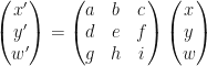
\begin{pmatrix}x^{\prime} \\ y^{\prime} \\ w^{\prime}\end{pmatrix}=\begin{pmatrix}a & b & c \\ d & e & f \\ g & h & i\end{pmatrix}\begin{pmatrix}x \\ y \\ w\end{pmatrix}

To get the 2D coordinates, we have to project back from 3D by dividing (x, y) by w. Since that division is a bit cumbersome, we will choose w=1. (The division makes sure w^{\prime}=1 too.) Let’s do a sanity check: a, b, d, e give the usual linear (2D) transformations, c, f give the translations, g, h give the projective transformations, and i is a global scaling. This last transformation is redundant for our purposes so we can set i=1.

Now, we have the right transformation tool. Why, you may ask? The answer is because this transformation matrix has 8 (unknown) parameters and given the 4 corners of the (source) quadrilateral & (destination) rectangle, we can write down 8 equations relating them. So 8 equations and 8 unknowns → any respectable linear algebra package should be able to do the ‘Maths’! (Caveat: You – How do you know the destination corners? Me – Well, that’s ‘beyond the scope’ of this post. You – $$$##%%^#)

Actually, we can do better than that. If one stares at those 8 equations long enough, one realizes that those equations can be solved analytically if the transformation is from a unit square to a given quadrilateral! You might be thinking that’s not too helpful; we want the reverse at the very least. Not quite! Because in image transformation business, if you think about it, “you don’t PUT the pixel, you GET the pixel”. (That’s my quote and you can fearlessly attribute it to me from now on. – Thanks.) For more discussion on this revelation, read this post.

So what we have to do now is simple:

  1. Get the 4 coordinates of the corners of the quadrilateral in the source image: X_q .
  2. Find the 8 parameters (a, \cdots, h) in the transformation matrix from the analytical solution for the coordinates X_q: T_s .
  3. Figure out the corners of the destination rectangle: X_r .
  4. Scale the transformation matrix in (x,y) direction appropriately so that the square scales to the required rectangle: T_r=T_s \cdot\text{diag}\left(\tfrac{1}{W}, \tfrac{1}{H}, 1\right) 
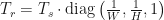
. (Width & Height are figured out from X_r.)
  5. Do the final transformation with translated coordinates: X_{\text{src}}=T_r \cdot (X_{\text{dest}}-X_{\text{trans}}) . (I find that incorporating the translations in the matrix is not that straightforward. Maybe it can be done, but translating the coordinates and then transforming them is simple enough. Also remember: “GET the Pixels”.)
  6. Crop the relevant portion of the transformed image.

After implementing the above algorithm, we can end up with something like this (I think the second last point becomes clear too):

Intermediary

Or to put it more bluntly, this:

Square

If you’re starting to think, I thought of all this… You’re giving me too much credit. Here’s the paper from where I learnt about this solution / algorithm (though, I think the solution given there may have some typos. I say this because that solution didn’t work ‘out of the box’):

Source

A Difficult Problem?

Many people land on this page of my other blog in search of an answer for this problem:

A circular lake 1.0 km in diameter is 10 m deep. Solar energy is incident on the lake at an average rate of 200 W/m². If the lake absorbs all this energy and does not exchange heat with its surroundings, how long will it take to warm from 10°C  to 20°C ?

as seen in the following snapshot:

Problem

Now, I do offer a pathway to the solution there but I feel that not providing the final answer is tantamount to cheating on my part. So, this being a ‘Physics blog’, I provide the entire solution here (I don’t know or care what good does it do to those ‘searchers’!):

t=\frac{Q}{S.A}=\frac{m.C.\Delta T}{S.A}=\frac{(\rho .V)C.\Delta T}{S.A}=\frac{\rho(A.h)C.\Delta T}{S.A}=\frac{\rho .h.C.\Delta T}{S}

\Rightarrow t=\frac{1000\times 10\times 4200\times (20-10)}{200}= 2.1\times 10^6s=24d~7h~20m.

3D Rotations

You should have come from here!

Here’s a quickie: What are the eigenvalues of a 2D rotation matrix?

Here’s a problem: For a bunch of rotations performed one after another on a 3D object, find an equivalent single rotation which would give the same result.

Here’s a solution: First of all, multiply all the rotation matrices (obviously!) such that R_{s}=R_{n}R_{n-1}\cdots R_{2}R_{1}. A single rotation is characterized by an axis and an angle of rotation. Let’s get the angle first. Find the eigenvalues of R_{s}. Two of them will be of the form: e^{\dot{\iota}\theta}\,\&\,e^{-\dot{\iota}\theta}
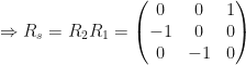
. This θ is the required angle. Let’s get the axis now. So what would be the third eigenvalue? Remember R_{s} \in SO(3) which means the third one is 1! Find the eigenvector corresponding to this eigenvalue which is the required axis!
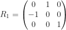
Here’s an example: Let’s do the problem mentioned in Gravitation.

R_{1}=\begin{pmatrix} 0 & 1 & 0 \\ -1 & 0 & 0 \\ 0 & 0 & 1 \end{pmatrix};

R_{2}=\begin{pmatrix} 0 & 0 & 1 \\ 0 & 1 & 0 \\ -1 & 0 & 0 \end{pmatrix}.

\Rightarrow R_{s}=R_{2}R_{1}=\begin{pmatrix} 0 & 0 & 1 \\ -1 & 0 & 0 \\ 0 & -1 & 0 \end{pmatrix}.

Relevant eigenvalues of R_{s} are -\frac{1}{2}\pm\frac{\sqrt{3}}{2}\dot{\iota} which give us the angle: \mathrm{tan}^{-1}\left(-\sqrt{3}\right)=120^{\circ}. The eigenvector corresponding to 1 is \frac{1}{\sqrt{3}}(1,-1,1) so the axis is one of the diagonals! This solution agrees with the one given in the book.